2c_plot_convergence.py — Plot Smearing Convergence
Plots the Allen-Feldman conductivity as a function of Lorentzian smearing η at each temperature. The plateau region in the plot identifies the physically meaningful smearing value to use in the final diffusivity calculation (step 3).
Output figures are saved to files (Agg backend; no display required).
Run after 2b_save_convergence.py.
cd tutorials/diffusivity
python 2c_plot_convergence.py
The output of the code will be a pdf containing the convergence plateau data at three temperatures: 100, 300 and 1500K:
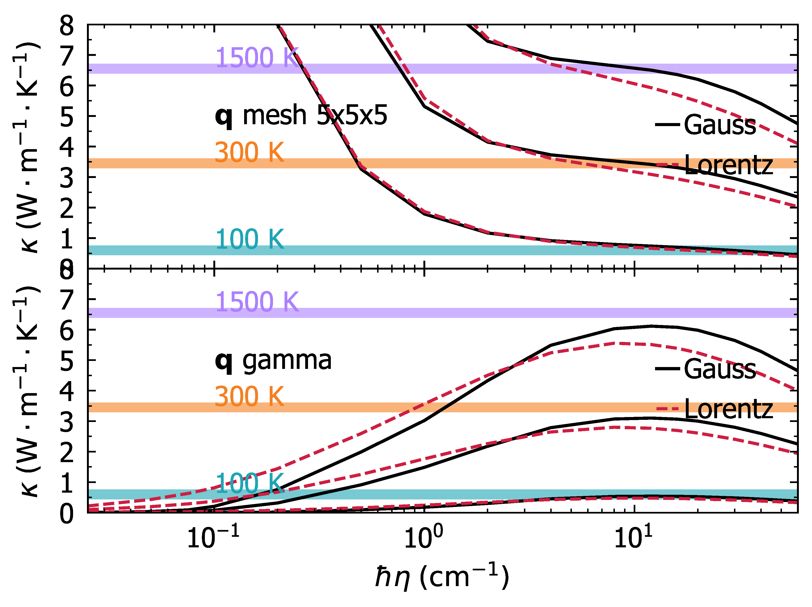
The smearing \(\eta\) value is chosen such that it is the lowest value at which
Allen-Feldman thermal conductivity is within the region of the convergence plateau (it converges).
For the IRG T9, the plateau at the gamma point is between ~7 to ~20 \(\text{cm}^{-1}\),
and on the 5×5×5 mesh between ~4 and ~12 \(\text{cm}^{-1}\), so the final chosen value of 8 \(\text{cm}^{-1}\)
is well within the convergence region (see gamma_min_plateau_cmm1 = 8.0 in the 3c_launch_serial.py script).
  1import string, re, struct, sys, math, os
  2import time
  3import types
  4from sys import argv
  5from shutil import move
  6from os import remove, close
  7from subprocess import PIPE, Popen
  8import numpy as np
  9import pandas as pd
 10import matplotlib
 11
 12# Use the non-interactive 'Agg' backend so figures are saved to files.
 13# This is needed on headless servers (no display) and for reproducible output.
 14matplotlib.use('Agg')
 15
 16import matplotlib.pyplot as pl
 17from mpl_toolkits.axes_grid1.inset_locator import inset_axes
 18from matplotlib import rc
 19from matplotlib import rcParams
 20from matplotlib.ticker import MultipleLocator, FormatStrFormatter
 21from scipy.optimize import curve_fit
 22from matplotlib import rc
 23from matplotlib import rcParams
 24from ase.io import read, write
 25from typing import Tuple
 26import scipy
 27
 28
 29# ---------------------------------------------------------------------------
 30# Font and LaTeX settings
 31# ---------------------------------------------------------------------------
 32
 33rcParams['font.family'] = 'sans-serif'
 34rcParams['font.sans-serif'] = ['Tahoma']   # Tahoma font matches the paper style
 35
 36matplotlib.rcParams.update({'font.size': 12})
 37
 38# LaTeX preamble: load siunitx for SI units and amsmath for equations
 39matplotlib.rcParams['text.latex.preamble'] = (
 40    r"\usepackage{siunitx} \sisetup{detect-all} \usepackage{amsmath, amssymb}"
 41)
 42
 43
 44
 45# ----------------------------------------
 46#              COLORS
 47# ---------------------------------------
 48
 49c_orange=np.array([172./255., 90./255., 22./255.,1.0])
 50c_red_nature=np.array([206./255., 30./255., 65./255.,1.0])
 51c_green_nature=np.array([96./255., 172./255., 63./255.,1.0])
 52c_blue_nature =np.array([54./255., 79./255., 156./255.,1.0])
 53c_purple_nature=np.array([245./255., 128./255., 32./255.,1.0])#np.array([192./255., 98./255., 166./255.,1.0])
 54c_black1=np.array([50./255., 50./255., 50./255.,1.0])
 55c_black2=np.array([100./255., 100./255.,100./255.,1.0])
 56c_black3=np.array([150./255., 150./255., 150./255.,1.0])
 57c_black4=np.array([200./255., 200./255., 200./255.,1.0])
 58c_cyna='#00aeff' #42cef4'
 59c_dark_green='#004d00'
 60c_pink='#ff1aff'
 61c_purple='#990099'
 62c_dark_orange='#db5f00'
 63c_orange='orange'
 64
 65
 66c_black=np.array([40./255., 41./255., 35./255.,1.0])
 67#c_black=np.array([116./255., 112./255., 93./255.,1.0])
 68
 69c_red=np.array([249./255., 36./255.,114./255.,1.0])
 70c_purple=np.array([172./255., 128./255., 255./255.,1.0])
 71c_orange=np.array([253./255., 150./255., 33./255.,1.0])
 72
 73
 74c_red=np.array([206./255., 30./255., 65./255.,1.0])
 75
 76#c_green=np.array([62./255., 208./255., 102./255.,1.0])
 77c_green=np.array([96./255., 172./255., 63./255.,1.0])
 78
 79c_blue=np.array([26./255., 97./255., 191./255.,1.0])
 80# c_pink=np.array([144./255., 110./255., 209./255.,1.0])#'#AE5BB3'  #F379FB'
 81c_orange=np.array([245./255., 128./255., 32./255.,1.0])
 82c_cyan=np.array([30./255., 165./255., 180./255.,1.0])
 83c_black=np.array([0./255., 0./255., 0./255.,1.0])
 84
 85
 86
 87# Unknown functions
 88def tc_composite(k_m, v_fra_air):
 89  k_eff=k_m*(2*k_m-2.*v_fra_air*k_m)/(2*k_m+v_fra_air*k_m)
 90  return k_eff
 91
 92def smoot_points(x,y,dense_x):
 93  spl=splrep(x,y,s=0.003)
 94  y2 = splev(dense_T, spl)
 95  return y2
 96
 97c_green=np.array([96./255., 172./255., 63./255.,1.0])
 98c_blue=np.array([26./255., 97./255., 191./255.,1.0])
 99
100class _Colors(object):
101    """Helper class with different colors for plotting"""
102    red = '#F15854'
103    blue = '#5DA5DA'
104    orange = '#FAA43A'
105    green = '#60BD68'
106    pink = '#F17CB0'
107    brown = '#B2912F'
108    purple = '#B276B2'
109    yellow = '#DECF3F'
110    gray = '#4D4D4D'
111    cyan = '#00FFFF'
112    rebecca_purple = '#663399'
113    chartreuse = '#7FFF00'
114    dark_red = '#8B0000'
115
116    def __getitem__(self, i):
117        color_list = [
118            self.red,
119            self.orange,
120            self.green,
121            self.blue,
122            self.pink,
123            self.brown,
124            self.purple,
125            self.yellow,
126            self.gray,
127            self.cyan,
128            self.rebecca_purple,
129            self.chartreuse,
130            self.dark_red
131        ]
132        return color_list[i % len(color_list)]
133
134
135Colors = _Colors()
136
137fig, (ax1, ax2) = pl.subplots(2, 1, sharex=True)
138fig.subplots_adjust(wspace=0, hspace=0)
139
140# read data
141directory = "."
142source = f"{directory}"
143kappas_G, kappas_L, kappas_G_gamma, kappas_L_gamma = \
144np.load(f"{source}/results/convergence_test.npy", allow_pickle=True)
145list_smear = [0.025, 0.05, 0.075, 0.1, 0.2, 0.5, 1.0, 2.0, 4.0, 8.0, 12.0, 16.0, 20.0, 30, 40, 60, 80, 100]
146temp_list = [100, 300, 1500]
147n_temp = len(temp_list)
148
149
150convergence_pos_y = [0.6, 3.45, 6.55]
151convergence_pos_x = [0.1, 0.1, 0.1]
152ylim = 8.0
153title_upper = [0.1, ylim/1.7, 13, 1.5]
154title_lower = [0.1, ylim/1.7, 1, 1.5]
155
156
157ax1.plot(list_smear, kappas_G[:, 0], label="Gauss", color=c_black, zorder=1)
158ax1.plot(list_smear, kappas_G[:, 1], color=c_black, zorder=1)
159ax1.plot(list_smear, kappas_G[:, 2], color=c_black, zorder=1)
160
161ax1.plot(list_smear, kappas_L[:, 0], label="Lorentz", color=c_red, linestyle='dashed', zorder=1)
162ax1.plot(list_smear, kappas_L[:, 1], color=c_red, linestyle='dashed', zorder=1)
163ax1.plot(list_smear, kappas_L[:, 2], color=c_red, linestyle='dashed', zorder=1)
164
165ax1.hlines(convergence_pos_y[2], list_smear[0], list_smear[-1], color=c_purple, zorder=0,alpha=0.6,lw=5)
166ax1.text(convergence_pos_x[2], convergence_pos_y[2]+0.05, f"{temp_list[2]} K", color=c_purple, fontsize=14)
167ax1.hlines(convergence_pos_y[1], list_smear[0], list_smear[-1], color=c_orange, zorder=0,alpha=0.6,lw=5)
168ax1.text(convergence_pos_x[1], convergence_pos_y[1]+0.05, f"{temp_list[1]} K", color=c_orange, fontsize=14)
169ax1.hlines(convergence_pos_y[0], list_smear[0], list_smear[-1], color=c_cyan, zorder=0,lw=5,alpha=0.6)
170ax1.text(convergence_pos_x[0], convergence_pos_y[0]+0.05, f"{temp_list[0]} K", color=c_cyan, fontsize=14)
171
172# ax1.vlines(3 * np.max(IC_datasets[0][3]) / (3 * 120), 0, 2.5, linestyle='dotted', color='grey')
173# ax1.text(10, 0.1, r'$3 \Delta \omega_{avg}$' ,fontsize=14)
174
175ax1.text(title_upper[0], title_upper[1], r'$\bf{q}$ mesh 5x5x5', fontsize=14)
176# ax1.text(title_upper[2], title_upper[3], structure_labels[structure_idx], fontsize=14)
177
178
179# set limits on x and y axes, ticks on axes, set scale to logs, set labels
180ax1.set_ylim([0., ylim])
181# ax1.
182# ax1.set_xticks(np.arange(0,40,2.5),minor=True)
183# ax1.set_xticks(np.arange(0,36,5),minor=False)
184ax1.set_yticks(np.arange(0, ylim+0.1, 0.5), minor=True)
185ax1.set_yticks(np.arange(0, ylim+0.1, 1.0), minor=False)
186
187# ax1.set_yscale('log')
188ax1.set_xscale('log')
189
190# ax1.set_xlabel(r'$\hbar \eta \;\left(\rm{cm}^{-1}\right)$',fontsize=14)
191ax1.set_ylabel(r'$\kappa \;\left(\rm{W} \cdot \rm{m}^{-1} \cdot \rm{K}^{-1}\right)$',fontsize=14, labelpad=8)
192
193
194handles, labels = ax1.get_legend_handles_labels()
195handles_mod=handles.copy()
196labels_mod=labels.copy()
197
198
199ax1.legend(loc='center right', fancybox=True, shadow=True, ncol=1, fontsize=14,
200          columnspacing=1.,scatterpoints=1,handletextpad=0.2,handlelength=0.8,frameon=False)
201
202ax1.tick_params(labelsize=14, direction='in',which='minor',bottom=True, top=True, left=True, right=True,length=2,pad=7)
203ax1.tick_params(labelsize=14, direction='in',which='major',bottom=True, top=True, left=True, right=True,length=4,pad=7)
204
205# --------------------------------- #
206
207ax2.plot(list_smear, kappas_G_gamma[:, 0], label="Gauss", color=c_black, zorder=1)
208ax2.plot(list_smear, kappas_G_gamma[:, 1], color=c_black, zorder=1)
209ax2.plot(list_smear, kappas_G_gamma[:, 2], color=c_black, zorder=1)
210
211
212ax2.plot(list_smear, kappas_L_gamma[:, 0], label="Lorentz", color=c_red, linestyle='dashed', zorder=1)
213ax2.plot(list_smear, kappas_L_gamma[:, 1], color=c_red, linestyle='dashed', zorder=1)
214ax2.plot(list_smear, kappas_L_gamma[:, 2], color=c_red, linestyle='dashed', zorder=1)
215
216
217ax2.hlines(convergence_pos_y[2], list_smear[0], list_smear[-1], color=c_purple, zorder=0,alpha=0.6,lw=5)
218ax2.text(convergence_pos_x[2], convergence_pos_y[2]+0.05, f"{temp_list[2]} K", color=c_purple, fontsize=14)
219ax2.hlines(convergence_pos_y[1], list_smear[0], list_smear[-1], color=c_orange, zorder=0,alpha=0.6,lw=5)
220ax2.text(convergence_pos_x[1], convergence_pos_y[1]+0.05, f"{temp_list[1]} K", color=c_orange, fontsize=14)
221ax2.hlines(convergence_pos_y[0], list_smear[0], list_smear[-1], color=c_cyan, zorder=0,lw=5,alpha=0.6)
222ax2.text(convergence_pos_x[0], convergence_pos_y[0]+0.05, f"{temp_list[0]} K", color=c_cyan, fontsize=14)
223
224# ax2.vlines(3 * np.max(IC_datasets[0][3]) / (3 * 120), 0, 2.5, linestyle='dotted', color='grey')
225# ax2.text(10, 0.1, r'$3 \Delta \omega_{avg}$' ,fontsize=14)
226
227ax2.text(title_lower[0], title_lower[1], r'$\bf{q}$ gamma', fontsize=14)
228# ax2.text(title_lower[2], title_lower[3], structure_labels[structure_idx], fontsize=14)
229
230# set limits on x and y axes, ticks on axes, set scale to logs, set labels
231ax2.set_ylim([0., ylim])
232ax2.set_xlim([0.025, 60])
233# ax2.set_xticks(np.arange(0,18,2.5),minor=True)
234# ax2.set_xticks(np.arange(0,16,5),minor=False)
235ax2.set_yticks(np.arange(0, ylim+0.1, 0.5), minor=True)
236ax2.set_yticks(np.arange(0, ylim+0.1, 1.0), minor=False)
237
238# ax2.set_yscale('log')
239# ax2.set_xscale('log')
240
241ax2.set_xlabel(r'$\hbar \eta \;\left(\rm{cm}^{-1}\right)$',fontsize=14)
242ax2.set_ylabel(r'$\kappa \;\left(\rm{W} \cdot \rm{m}^{-1} \cdot \rm{K}^{-1}\right)$',fontsize=14, labelpad=8)
243
244
245handles, labels = ax2.get_legend_handles_labels()
246handles_mod=handles.copy()
247labels_mod=labels.copy()
248
249
250ax2.legend(loc='center right', fancybox=True, shadow=True, ncol=1, fontsize=14,
251          columnspacing=1.,scatterpoints=1,handletextpad=0.2,handlelength=0.8,frameon=False)
252
253ax2.tick_params(labelsize=14, direction='in',which='minor',bottom=True, top=True, left=True, right=True,length=2,pad=7)
254ax2.tick_params(labelsize=14, direction='in',which='major',bottom=True, top=True, left=True, right=True,length=4,pad=7)
255
256
257save_directory = "."
258name_file_save=f't9_216_convergence_test.pdf'
259scale = 1.
260fig.set_size_inches(6.5*scale, 4.5*scale)
261fig.savefig(save_directory + "/" + name_file_save, dpi=300, bbox_inches="tight",transparent=True)