Notebook 4 — Bond-Network Entropy

What we do here

We now compute the Bond-Network Entropy (BNE) of the silica glass. The idea:

1. Compute the H₁ barcode for every atom’s local environment (LAE size = 30).

2. Group atoms by barcode — identical barcodes form an equivalence class.

3. Compute the empirical probability \(p_m\) of each class.

4. Apply information entropy to the class distribution.

Reference: K. Iwanowski, G. Csányi, and M. Simoncelli, Phys. Rev. X 15, 041041 (2025)

---

Theory: Shannon entropy and Bond-Network Entropy

Shannon entropy measures the diversity of a probability distribution. Given classes with probabilities \(p_1, p_2, \ldots, p_k\) (with \(\sum_m p_m = 1\)):

\[S = -\sum_m p_m \ln p_m\]

• If one class dominates (\(p_1 \approx 1\)): \(S \approx 0\) — almost all atoms have the same environment, highly ordered.

• If all classes are equally likely (\(p_m = 1/k\)): \(S = \ln k\) — maximum heterogeneity.

BNE applies this formula to the distribution of H₁ barcodes across all atoms. A higher BNE means the bond network has greater topological diversity — more disorder.

The BNE depends on the LAE size \(n\). We fix \(n = 30\) here (a good compromise: large enough to capture ring structure, small enough to compute quickly and avoid saturation effects). Notebook 6 explores how BNE changes with \(n\).

The normalised growth rate BNE\((n)/n\) is a material fingerprint that allows distinguishing different materials based on the level of disorder in their bond network.

Library and visualization setup

import os, sys

import numpy as np
import pandas as pd
import scipy
from scipy.constants import physical_constants

import ase
from ase.io import read, write

matplotlib_style = 'fivethirtyeight'
import matplotlib.pyplot as plt
plt.style.use(matplotlib_style)
import seaborn as sns
sns.set_context('notebook')

class _Colors(object):
    """Helper class with different colors for plotting"""
    red = '#F15854'
    blue = '#5DA5DA'
    orange = '#FAA43A'
    green = '#60BD68'
    pink = '#F17CB0'
    brown = '#B2912F'
    purple = '#B276B2'
    yellow = '#DECF3F'
    gray = '#4D4D4D'
    cyan = '#00FFFF'
    rebecca_purple = '#663399'
    chartreuse = '#7FFF00'
    dark_red = '#8B0000'

    def __getitem__(self, i):
        color_list = [
            self.red,
            self.orange,
            self.green,
            self.blue,
            self.pink,
            self.brown,
            self.purple,
            self.yellow,
            self.gray,
            self.cyan,
            self.rebecca_purple,
            self.chartreuse,
            self.dark_red
        ]
        return color_list[i % len(color_list)]


Colors = _Colors()

from typing import Tuple, List
from tqdm import tqdm

# handy function to obtain distances to nearest atoms (distances) and their indices (idx_distances)

def obtain_distances_ase(
    atoms: ase.atoms.Atoms,
    n_smallest: int,
) -> Tuple[np.ndarray, np.ndarray]:
    """
    Compute the n_smallest nearest-neighbour distances for every atom using
    the ASE Minimum Image Convention (preferred method).

    ASE's ``get_distances`` method handles the MIC correctly for all cell
    shapes (orthorhombic, monoclinic, triclinic), making it more accurate
    than the manual implementation for non-cubic cells.

    Parameters
    ----------
    atoms : ase.atoms.Atoms
        ASE Atoms object containing positions and cell (lattice vectors).
        Load from file with ``ase.io.read(filename)``.
    n_smallest : int
        Number of nearest neighbours (including central atom) to keep per atom.

    Returns
    -------
    distances : np.ndarray, shape (N, n_smallest)
        Sorted nearest-neighbour distances (in Ångström).
    idx_distances : np.ndarray, shape (N, n_smallest)
        Global atom indices corresponding to those distances.
    """

    distances = []
    idx_distances = []

    nat = len(atoms)
    atom_indices = np.arange(0, nat, 1)

    for k in tqdm(range(len(atoms)), desc="Distances"):

        # ASE computes MIC-corrected distances from atom k to all others
        distance = atoms.get_distances(k, atom_indices, mic=True)

        # keep only the n_smallest nearest neighbours using argpartition
        if n_smallest < nat:
            idx_distance = np.argpartition(distance, n_smallest)[:n_smallest]
        else:
            idx_distance = np.arange(0, nat, 1)

        # sort by distance within the selected neighbours
        idx_distance = idx_distance[np.argsort(distance[idx_distance])]

        idx_distances.append(idx_distance)
        distances.append(distance[idx_distance])

    distances = np.array(distances)
    idx_distances = np.array(idx_distances)
    return distances, idx_distances

from smooth_disorder.barcode import (
    obtain_local_number_environment_big_structures,
    obtain_H1_barcode,
    reduce_barcode,
    mu,
)

import networkx as nx

%%time
# read structure downloaded from https://www.pnas.org/doi/abs/10.1073/pnas.2422763122
filename = "./data/structural/silica_glass_5184_atoms/POSCAR"

atoms = read(filename)

atomic_numbers = atoms.get_atomic_numbers()

distances, idx_distances = obtain_distances_ase(atoms, 300)

Distances: 100%|███████████████████████████████████████████████████████████████████████████████████████████████████████████████████████████████████████████████████████| 5184/5184 [00:13<00:00, 375.79it/s]

CPU times: user 11.5 s, sys: 4.53 s, total: 16.1 s
Wall time: 13.8 s

cutoff = 2.1 # for silica
adjacency_matrix = ((distances < cutoff) & (distances > 0.1)).astype(int)
coordination_number = adjacency_matrix.sum(axis=1)

Calculate Bond-Network Entropy for the material

We define a helper function calculate_barcode_distribution that, given an LAE size, loops over all atoms and returns the barcode equivalence classes and their counts. This makes it easy to reuse for different \(n\) values later.

Timing note: The cell after this one loops over all 5184 atoms, computing one H₁ barcode per atom. With LAE size 30 this takes approximately 15–60 seconds on a laptop. The %%time command will show the exact duration.

def calculate_barcode_distribution(distances, idx_distances, adjacency_matrix, n_atoms, LAE_size):
    """
    Compute the H1 barcode for every atom's local environment and return
    the unique barcode classes with their counts.

    Parameters
    ----------
    distances : ndarray, shape (N, K)
        Sorted pairwise distances from obtain_distances_ase.
    idx_distances : ndarray, shape (N, K)
        Corresponding atom indices.
    adjacency_matrix : ndarray, shape (N, K)
        Compressed adjacency matrix (1 = bonded).
    n_atoms : int
        Total number of atoms.
    LAE_size : int
        Number of atoms in each local atomic environment.

    Returns
    -------
    Gs : dict
        Barcode arrays grouped by matrix shape.
    class_counts : ndarray
        Count of atoms in each barcode equivalence class.
    probabilities : ndarray
        Empirical probability of each class (sums to 1).
    entropy : float
        Shannon entropy of the class distribution (in nats).
    """
    shapes = {}
    Gs = {}

    for atom_index in tqdm(range(n_atoms), desc=f"LAE size {LAE_size}"):
        local_adj, layers, local_idx, global_idx = obtain_local_number_environment_big_structures(
            adjacency_matrix=adjacency_matrix,
            atom_index=atom_index,
            distances=distances,
            idx_distances=idx_distances,
            n_environment_atoms=LAE_size)

        G, F = obtain_H1_barcode(adjacency_matrix=local_adj, layers=layers, mu=mu)
        G = reduce_barcode(G)

        shape = G.shape
        if shape not in shapes:
            shapes[shape] = 1
            Gs[shape] = []
        Gs[shape].append(G)

    # Collect equivalence class counts across all shapes
    class_counts = []
    for shape, gs in Gs.items():
        _, counts = np.unique(gs, return_counts=True, axis=0)
        class_counts.extend(counts)

    class_counts = np.array(class_counts)
    probabilities = class_counts / class_counts.sum()
    entropy = -(probabilities * np.log(probabilities)).sum()

    return Gs, class_counts, probabilities, entropy

%%time
LE_nat = 30
n_atoms = len(atoms)

Gs, class_counts, probabilities, entropy = calculate_barcode_distribution(
    distances, idx_distances, adjacency_matrix, n_atoms, LE_nat
)

LAE size 30: 100%|█████████████████████████████████████████████████████████████████████████████████████████████████████████████████████████████████████████████████████| 5184/5184 [00:19<00:00, 270.41it/s]

CPU times: user 19.1 s, sys: 83 ms, total: 19.2 s
Wall time: 19.2 s

print(f"BNE (n={LE_nat}): {entropy:.4f} nats")
print(f"BNE / n = {entropy/LE_nat:.4f} nats per atom")

BNE (n=30): 4.1477 nats
BNE / n = 0.1383 nats per atom

\({\rm BNE}(n)/n \approx 0.14\) nats per atom. What does this number mean?

For reference, different materials span a range of BNE growth rates:

• Crystalline material — all atoms identical → \({\rm BNE}(n)/n \approx 0\) (all barcodes the same)

• Disordered carbon — \(\text{BNE}(n)/n\) varies between 0.05 (low-irradiated graphite), 0.1 (low-disordered nanoporous carbon), 0.15 (medium-disordered nanoporous carbon), 0.2 (heavily-disordered nanoporous carbon), 0.25 (amorphous carbon)

Silica glass has very little coordination-number disorder but a non-zero bond-network disorder — BNE captures the latter, which simpler descriptors miss.

# Ranked distribution of barcode probabilities
# Each point is one equivalence class of barcodes; the x-axis ranks them by frequency

plt.figure(figsize=(16, 8))
plt.scatter(np.arange(1, len(probabilities)+1, 1), np.sort(probabilities)[::-1])
plt.xlabel("Barcode rank (most common = 1)")
plt.ylabel("Fraction of atoms with this barcode")
plt.title(f"Barcode probability distribution — LAE size {LE_nat}")

plt.xscale('log')
plt.yscale('log')

plt.show()

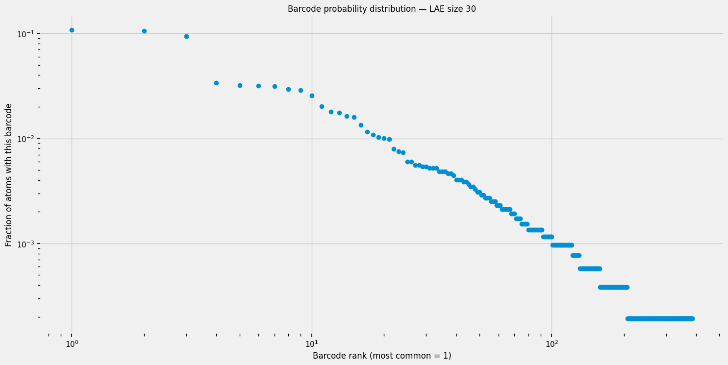
The 3 most common barcodes take about 30% of the distribution, let’s find how they look like:

common_barcodes, common_barcode_counts = [], []

for shape, gs in Gs.items():
    equivalence_class, class_count = np.unique(gs, return_counts=True, axis=0)
    common_barcodes.append(equivalence_class[class_count > 0.06*n_atoms])
    common_barcode_counts.append(class_count[class_count > 0.06*n_atoms])

# Print the three most common barcodes and their counts
for barcode_group, count_group in zip(common_barcodes, common_barcode_counts):
    for b, c in zip(barcode_group, count_group):
        print(f"Count: {c}  ({100*c/n_atoms:.1f}%)")
        print(f"Barcode:\n{b}\n")

Count: 487  (9.4%)
Barcode:
[[0. 0. 0. 0. 0. 1.]
 [0. 0. 0. 0. 0. 0.]
 [0. 0. 0. 0. 0. 0.]
 [0. 0. 0. 0. 0. 0.]
 [0. 0. 0. 0. 0. 0.]
 [0. 0. 0. 0. 0. 0.]]

Count: 548  (10.6%)
Barcode:
[[0. 0. 0. 0. 1.]
 [0. 0. 0. 0. 0.]
 [0. 0. 0. 0. 0.]
 [0. 0. 0. 0. 0.]
 [0. 0. 0. 0. 0.]]

Count: 560  (10.8%)
Barcode:
[[0.]]

The three most common barcodes collectively account for ~30% of all atoms.

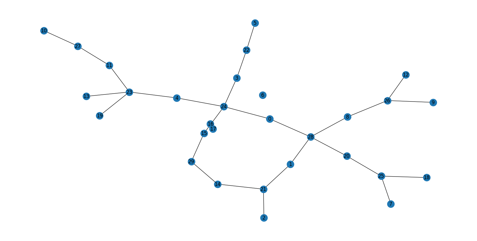
• [[0.]] (null barcode) — no rings in the 30-atom environment (the most common)

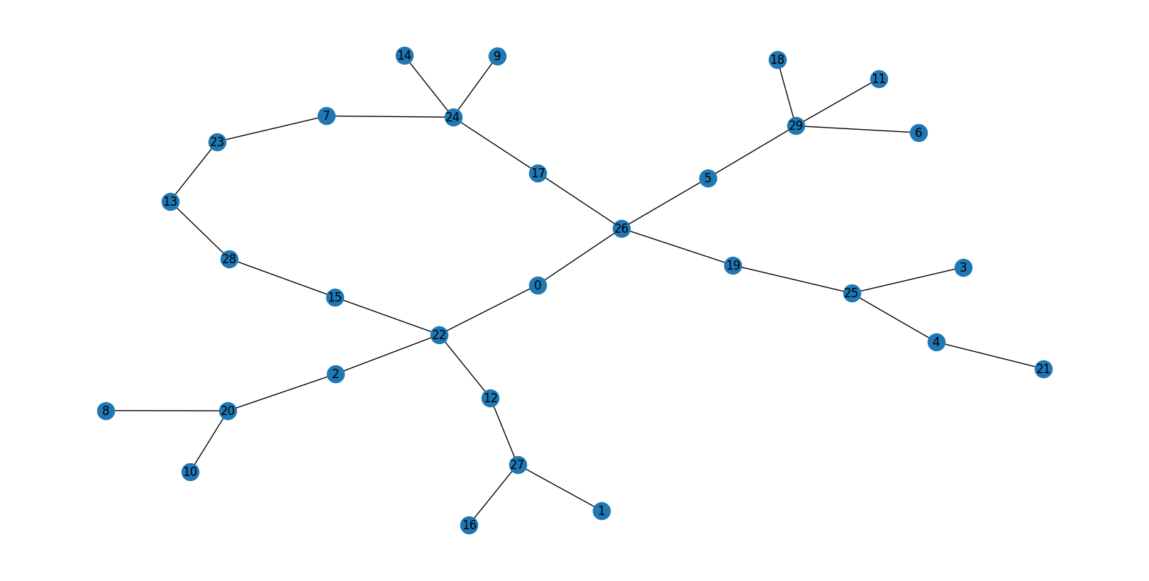
• Single bar at [0,4] — one ring closing at 4 hops from centre

• Single bar at [0,5] — one ring closing at 5 hops from centre

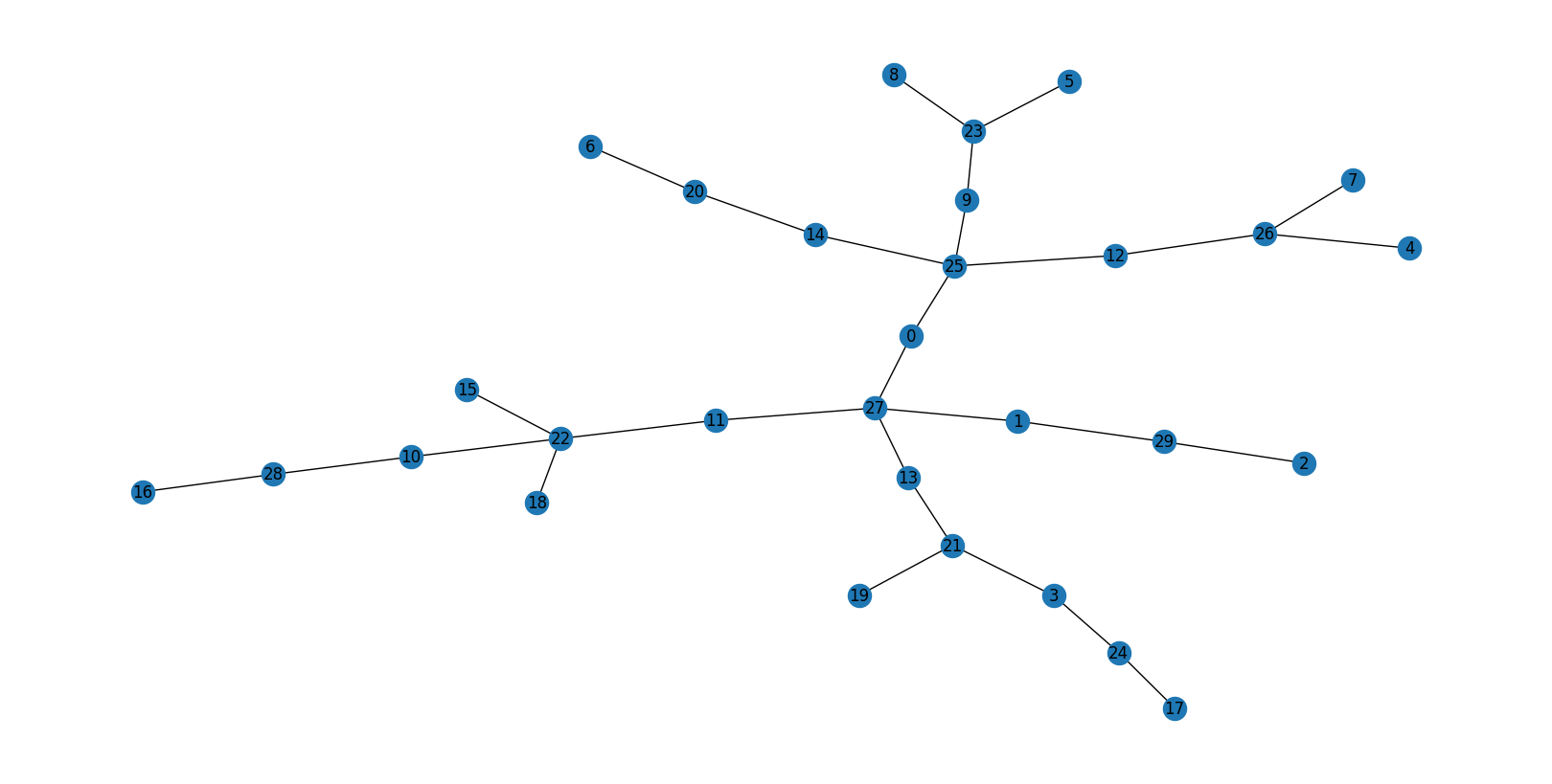
Let’s visualise one representative atom for each of these three barcode types:

LE_nat = 30

for atom_index in range(0, n_atoms):
    local_adjacency_matrix, layers, local_atom_index, global_index = obtain_local_number_environment_big_structures(
        adjacency_matrix=adjacency_matrix,
        atom_index=atom_index,
        distances=distances,
        idx_distances=idx_distances,
        n_environment_atoms=LE_nat)

    G, F = obtain_H1_barcode(adjacency_matrix=local_adjacency_matrix,
                             layers=layers,
                             mu=mu)

    G = reduce_barcode(G)

    if np.array_equal(G, np.array([[0.]])):
        print(atom_index)
        break

25

atom_index = 25
LAE_size = 30

local_adjacency_matrix, layers, local_atom_index, global_index = obtain_local_number_environment_big_structures(adjacency_matrix,
                                                                                                               atom_index,
                                                                                                               distances,
                                                                                                               idx_distances,
                                                                                                               LAE_size)

print(local_atom_index)

G, F = obtain_H1_barcode(adjacency_matrix=local_adjacency_matrix,
                         layers=layers,
                         mu=mu)

G = reduce_barcode(G)
print(G)

graph = nx.from_numpy_array(local_adjacency_matrix)

plt.figure(figsize=(16, 8))
pos = nx.kamada_kawai_layout(graph)
nx.draw(graph, pos=pos, with_labels=True)
plt.show()
# no rings

0
[[0.]]

LE_nat = 30

for atom_index in range(0, n_atoms):
    local_adjacency_matrix, layers, local_atom_index, global_index = obtain_local_number_environment_big_structures(
        adjacency_matrix=adjacency_matrix,
        atom_index=atom_index,
        distances=distances,
        idx_distances=idx_distances,
        n_environment_atoms=LE_nat)

    G, F = obtain_H1_barcode(adjacency_matrix=local_adjacency_matrix,
                             layers=layers,
                             mu=mu)

    G = reduce_barcode(G)

    if np.array_equal(G, np.array([[0., 0., 0., 0., 1.],
                                   [0., 0., 0., 0., 0.],
                                   [0., 0., 0., 0., 0.],
                                   [0., 0., 0., 0., 0.],
                                   [0., 0., 0., 0., 0.]])):
        print(atom_index)
        break

7

atom_index = 7
LAE_size = 30

local_adjacency_matrix, layers, local_atom_index, global_index = obtain_local_number_environment_big_structures(adjacency_matrix,
                                                                                                               atom_index,
                                                                                                               distances,
                                                                                                               idx_distances,
                                                                                                               LAE_size)

print(local_atom_index)

G, F = obtain_H1_barcode(adjacency_matrix=local_adjacency_matrix,
                         layers=layers,
                         mu=mu)

G = reduce_barcode(G)
print(G)

graph = nx.from_numpy_array(local_adjacency_matrix)

plt.figure(figsize=(16, 8))
pos = nx.kamada_kawai_layout(graph)
nx.draw(graph, pos=pos, with_labels=True)
plt.show()
# 1 [0, 4] ring

0
[[0. 0. 0. 0. 1.]
 [0. 0. 0. 0. 0.]
 [0. 0. 0. 0. 0.]
 [0. 0. 0. 0. 0.]
 [0. 0. 0. 0. 0.]]

LE_nat = 30

for atom_index in range(0, n_atoms):
    local_adjacency_matrix, layers, local_atom_index, global_index = obtain_local_number_environment_big_structures(
        adjacency_matrix=adjacency_matrix,
        atom_index=atom_index,
        distances=distances,
        idx_distances=idx_distances,
        n_environment_atoms=LE_nat)

    G, F = obtain_H1_barcode(adjacency_matrix=local_adjacency_matrix,
                             layers=layers,
                             mu=mu)

    G = reduce_barcode(G)

    if np.array_equal(G, np.array([[0., 0., 0., 0., 0., 1.],
                                   [0., 0., 0., 0., 0., 0.],
                                   [0., 0., 0., 0., 0., 0.],
                                   [0., 0., 0., 0., 0., 0.],
                                   [0., 0., 0., 0., 0., 0.],
                                   [0., 0., 0., 0., 0., 0.]])):
        print(atom_index)
        break

0

atom_index = 0
LAE_size = 30

local_adjacency_matrix, layers, local_atom_index, global_index = obtain_local_number_environment_big_structures(adjacency_matrix,
                                                                                                               atom_index,
                                                                                                               distances,
                                                                                                               idx_distances,
                                                                                                               LAE_size)

print(local_atom_index)

G, F = obtain_H1_barcode(adjacency_matrix=local_adjacency_matrix,
                         layers=layers,
                         mu=mu)

G = reduce_barcode(G)
print(G)

graph = nx.from_numpy_array(local_adjacency_matrix)

plt.figure(figsize=(16, 8))
pos = nx.kamada_kawai_layout(graph)
nx.draw(graph, pos=pos, with_labels=True)
plt.show()
# 1 [0, 5] ring

0
[[0. 0. 0. 0. 0. 1.]
 [0. 0. 0. 0. 0. 0.]
 [0. 0. 0. 0. 0. 0.]
 [0. 0. 0. 0. 0. 0.]
 [0. 0. 0. 0. 0. 0.]
 [0. 0. 0. 0. 0. 0.]]

BNE depends on the LAE size — a preview

Everything computed above uses LAE size \(n = 30\). But BNE is not fixed: as we include more distant atoms in each environment, we discover more rings, we are able to distinguish environments and the entropy grows.

The theoretical maximum BNE is \(S_{\max} = \ln(N)\) — reached only if every one of the \(N = 5184\) atoms had a completely unique barcode. For silica, \(\ln(5184) \approx 8.55\) nats.

In practice BNE grows roughly linearly with \(n\) in an intermediate range, then saturates as most atoms have distinct environments at very large \(n\). The growth rate BNE\((n)/n\) in the linear regime is the material fingerprint.

Notebook 5 (5_BNE_workflow.py) computes BNE for \(n = 1, 2, \ldots, 80\) and saves the results to HDF5 files (these are precomputed in this tutorial). Notebook 6 then plots the growth curve and extracts the growth rate.