Notebook 6 — BNE Growth Rate and Saturation

What we do here

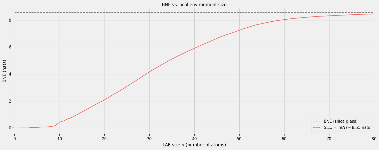
In Notebook 4 we computed BNE for a single LAE size (\(n = 30\)). Here we load the pre-computed BNE values for \(n = 1, 2, \ldots, 80\) (computed by 5_BNE_workflow.py) and analyse how BNE grows with \(n\).

Reference: K. Iwanowski, G. Csányi, and M. Simoncelli, Phys. Rev. X 15, 041041 (2025)

---

Theory: growth rate and saturation

As we increase the LAE size \(n\):

• At small :math:`n`: most atoms see identical tiny environments → BNE is small.

• At intermediate :math:`n`: the number of distinct ring environments grows roughly exponentially, BNE grows linearly. The slope BNE\((n)/n\) in this regime is the material fingerprint.

• At large :math:`n`: the environment is so big that local environments become unique, so BNE saturates.

The theoretical maximum is \(S_{\max} = \ln(N)\), reached if every atom had a completely unique barcode. For \(N = 5184\) atoms: \(\ln(5184) \approx 8.55\) nats.

The function normalised_BNE estimates the growth rate by averaging BNE\((n)/n\) over a range \([n_{\rm start}, n_{\rm stop}]\) that sits in the linear regime (avoiding the early transient at small \(n\) and the saturation effects at large \(n\)).

import os, sys

import numpy as np
import pandas as pd
import scipy
from scipy.constants import physical_constants

import ase
from ase.io import read, write

matplotlib_style = 'fivethirtyeight'
import matplotlib.pyplot as plt
plt.style.use(matplotlib_style)
import seaborn as sns
sns.set_context('notebook')

class _Colors(object):
    """Helper class with different colors for plotting"""
    red = '#F15854'
    blue = '#5DA5DA'
    orange = '#FAA43A'
    green = '#60BD68'
    pink = '#F17CB0'
    brown = '#B2912F'
    purple = '#B276B2'
    yellow = '#DECF3F'
    gray = '#4D4D4D'
    cyan = '#00FFFF'
    rebecca_purple = '#663399'
    chartreuse = '#7FFF00'
    dark_red = '#8B0000'

    def __getitem__(self, i):
        color_list = [
            self.red,
            self.orange,
            self.green,
            self.blue,
            self.pink,
            self.brown,
            self.purple,
            self.yellow,
            self.gray,
            self.cyan,
            self.rebecca_purple,
            self.chartreuse,
            self.dark_red
        ]
        return color_list[i % len(color_list)]


Colors = _Colors()

from typing import Tuple, List
from tqdm import tqdm

import h5py

BNE_data_directory = "./data/bond_network_entropy"

BNE_data = {}

structure_idx = 0

temp_BNE = []
temp_nat = []
for LE_nat in range(1, 81):
    with h5py.File(f"{BNE_data_directory}/structure_{structure_idx}/entropy_number_{LE_nat}.hdf5", "r") as f:
        temp_BNE.append(np.asarray(f['entropy'])[0])
        temp_nat.append(np.asarray(f['number_of_atoms'])[0])

temp_BNE, temp_nat = np.array(temp_BNE), np.array(temp_nat)

BNE_data[f"{structure_idx}_BNE"] = temp_BNE
BNE_data[f"{structure_idx}_nat"] = temp_nat

n_start, n_stop = 10, 40

def normalised_BNE(n_atoms, entropy, n_start=n_start, n_stop=n_stop):
    """
    Estimate the BNE growth rate by averaging BNE(n)/n over [n_start, n_stop].

    n_start=10 avoids the early transient (small environments
    look identical); n_stop=40 avoids the saturation regime (large environments
    start to become unique, bending the curve).

    Returns
    -------
    BNE_mean : float
        Mean BNE(n)/n in nats per atom — the growth rate estimate.
    BNE_std : float
        Standard deviation of BNE(n)/n over the window.
    """
    idx_start = np.arange(0, len(n_atoms), 1)[n_atoms == n_start][-1]
    idx_stop  = np.arange(0, len(n_atoms), 1)[n_atoms == n_stop][0]

    local_n_atoms  = n_atoms[idx_start:idx_stop+1]
    local_quotient = entropy[idx_start:idx_stop+1] / local_n_atoms

    BNE_mean = np.mean(local_quotient)
    BNE_std  = np.std(local_quotient, ddof=1)

    return BNE_mean, BNE_std

n_atoms_silica = 5184
S_max = np.log(n_atoms_silica)  # theoretical maximum BNE

structure_idx = 0
nat  = BNE_data[f"{structure_idx}_nat"]
bne  = BNE_data[f"{structure_idx}_BNE"]

plt.figure(figsize=(16, 6))
plt.plot(nat, bne, color=Colors[0], label="BNE (silica glass)")
plt.axhline(S_max, color='gray', linestyle='--', label=rf"$S_{{\max}} = \ln(N) \approx {S_max:.2f}$ nats")
plt.ylabel("BNE (nats)")
plt.xlabel("LAE size $n$ (number of atoms)")
plt.xlim([0, 80])
plt.legend()
plt.title("BNE vs local environment size")
plt.show()

bne_mean, bne_std = normalised_BNE(nat, bne)
print(f"Growth rate (BNE/n averaged over n={n_start}–{n_stop}): {bne_mean:.4f} ± {bne_std:.4f} nats/atom")

Growth rate (BNE/n averaged over n=10–40): 0.1139 ± 0.0327 nats/atom

Where does BNE saturate?

From the plot above, BNE grows roughly linearly up to \(n \approx 50\), after which the curve clearly bends over and approaches \(S_{\max}\). By \(n = 80\), BNE \(\approx 8.45\) nats, within \(\sim 0.1\) nats of the ceiling \(S_{\max} = \ln(N) \approx 8.55\) nats — saturation is essentially complete.

By linearly extrapolating the growth rate (estimated in the \(n = 10\)–\(40\) linear regime) to the saturation ceiling, we can estimate the LAE size \(n^*\) at which saturation occurs:

\[n^* \approx \frac{S_{\max}}{\text{growth rate}} = \frac{\ln(N)}{\text{BNE}(n)/n}\]

For silica, this predicts \(n^* \approx 75\) atoms, consistent with what we see in the data: the curve has nearly reached \(S_{\max}\) by \(n = 75\)–\(80\).

n_star = S_max / bne_mean
print(f"Estimated saturation LAE size: n* ≈ {n_star:.0f} atoms")
print(f"(where the linear extrapolation reaches S_max = ln({n_atoms_silica}) = {S_max:.2f} nats)")

Estimated saturation LAE size: n* ≈ 75 atoms
(where the linear extrapolation reaches S_max = ln(5184) = 8.55 nats)