Notebook 2 — Coordination Number Distribution

What we do here

In Notebook 1 we computed pairwise distances with the Minimum Image Convention. Now we:

1. Build the adjacency matrix — the graph representation of the bond network.

2. Count coordination numbers and visualise their distribution.

---

The bond network as a graph

We represent the atomic structure as a graph where:

• Nodes = atoms (5184 total: 3456 O + 1728 Si)

• Edges = bonds (pairs of atoms within the cutoff distance)

The adjacency matrix \(A\) encodes the bonds: \(A_{ij} = 1\) if atoms \(i\) and \(j\) are bonded, \(A_{ij} = 0\) otherwise.

Because we store only the n_smallest = 300 nearest neighbours per atom (from Notebook 1), \(A\) has a compressed shape (N_atoms, 300) rather than a full (N_atoms, N_atoms) matrix. Entry A[i, k] = 1 means atom \(i\) is bonded to atom idx_distances[i, k].

The coordination number of atom \(i\) is the degree of its node in the graph: \(z_i = \sum_k A_{ik}\).

For a perfect SiO₂ glass, we expect \(z = 2\) for oxygen (bridging) and \(z = 4\) for silicon (tetrahedral SiO₄ units). Deviations indicate defects or disorder.

Library + visualization setup

import os, sys

import numpy as np
import pandas as pd
import scipy
from scipy.constants import physical_constants

import ase
from ase.io import read, write

matplotlib_style = 'fivethirtyeight'
import matplotlib.pyplot as plt
plt.style.use(matplotlib_style)
import seaborn as sns
sns.set_context('notebook')

class _Colors(object):
    """Helper class with different colors for plotting"""
    red = '#F15854'
    blue = '#5DA5DA'
    orange = '#FAA43A'
    green = '#60BD68'
    pink = '#F17CB0'
    brown = '#B2912F'
    purple = '#B276B2'
    yellow = '#DECF3F'
    gray = '#4D4D4D'
    cyan = '#00FFFF'
    rebecca_purple = '#663399'
    chartreuse = '#7FFF00'
    dark_red = '#8B0000'

    def __getitem__(self, i):
        color_list = [
            self.red,
            self.orange,
            self.green,
            self.blue,
            self.pink,
            self.brown,
            self.purple,
            self.yellow,
            self.gray,
            self.cyan,
            self.rebecca_purple,
            self.chartreuse,
            self.dark_red
        ]
        return color_list[i % len(color_list)]


Colors = _Colors()

from typing import Tuple, List
from tqdm import tqdm

# handy function to obtain distances to nearest atoms (distances) and their indices (idx_distances)

def obtain_distances_ase(
    atoms: ase.atoms.Atoms,
    n_smallest: int,
) -> Tuple[np.ndarray, np.ndarray]:
    """
    Compute the n_smallest nearest-neighbour distances for every atom using
    the ASE Minimum Image Convention (preferred method).

    ASE's ``get_distances`` method handles the MIC correctly for all cell
    shapes (orthorhombic, monoclinic, triclinic), making it more accurate
    than the manual implementation for non-cubic cells.

    Parameters
    ----------
    atoms : ase.atoms.Atoms
        ASE Atoms object containing positions and cell (lattice vectors).
        Load from file with ``ase.io.read(filename)``.
    n_smallest : int
        Number of nearest neighbours (including central atom) to keep per atom.

    Returns
    -------
    distances : np.ndarray, shape (N, n_smallest)
        Sorted nearest-neighbour distances (in Ångström).
    idx_distances : np.ndarray, shape (N, n_smallest)
        Global atom indices corresponding to those distances.
    """

    distances = []
    idx_distances = []

    nat = len(atoms)
    atom_indices = np.arange(0, nat, 1)

    for k in tqdm(range(len(atoms)), desc="Distances"):

        # ASE computes MIC-corrected distances from atom k to all others
        distance = atoms.get_distances(k, atom_indices, mic=True)

        # keep only the n_smallest nearest neighbours using argpartition
        if n_smallest < nat:
            idx_distance = np.argpartition(distance, n_smallest)[:n_smallest]
        else:
            idx_distance = np.arange(0, nat, 1)

        # sort by distance within the selected neighbours
        idx_distance = idx_distance[np.argsort(distance[idx_distance])]

        idx_distances.append(idx_distance)
        distances.append(distance[idx_distance])

    distances = np.array(distances)
    idx_distances = np.array(idx_distances)
    return distances, idx_distances

Load the structure and compute distances

Timing note: obtain_distances_ase loops over all atoms with ASE’s MIC routine. This takes 15-30 seconds on a typical laptop.

%%time
# read structure downloaded from https://www.pnas.org/doi/abs/10.1073/pnas.2422763122
filename = "./data/structural/silica_glass_5184_atoms/POSCAR"

atoms = read(filename)

atomic_numbers = atoms.get_atomic_numbers()

distances, idx_distances = obtain_distances_ase(atoms, 300)

Distances: 100%|███████████████████████████████████████████████████████████████████████████████████████████████████████████████████████████████████████████████████████| 5184/5184 [00:14<00:00, 366.02it/s]

CPU times: user 11.7 s, sys: 4.7 s, total: 16.4 s
Wall time: 14.2 s

Building the adjacency matrix and coordination numbers

Now we apply the bond cutoff to build \(A\):

cutoff = 2.1  # Å — Si–O nearest-neighbour bond cutoff for silica glass

# A[i, k] = 1 if atom i is bonded to its k-th stored neighbour
# The lower bound (> 0.1 Å) excludes the self-distance at d = 0
adjacency_matrix = ((distances < cutoff) & (distances > 0.1)).astype(int)

# Coordination number = number of bonds per atom (row sum)
coordination_number = adjacency_matrix.sum(axis=1)

oxygen_unique, oxygen_counts = np.unique(coordination_number[atomic_numbers == 8], return_counts=True)
oxygen_unique

array([1, 2, 3])

oxygen_counts

array([   1, 3453,    2])

silicon_unique, silicon_counts = np.unique(coordination_number[atomic_numbers == 14], return_counts=True)
silicon_unique

array([3, 4, 5])

silicon_counts

array([   2, 1723,    3])

# figure similar to Fig. 1 of https://journals.aps.org/prmaterials/abstract/10.1103/PhysRevMaterials.8.043601

plt.figure(figsize=(16, 8))

plt.bar(oxygen_unique-0.05, oxygen_counts/oxygen_counts.sum(), width=0.1 , color=Colors[0], label='oxygen')
plt.bar(silicon_unique+0.05, silicon_counts/silicon_counts.sum(), width=0.1 , color=Colors[2], label='silicon')

plt.ylabel("Probability")
plt.xlabel("Coordination number")

plt.legend()
plt.yscale('log')

plt.show()

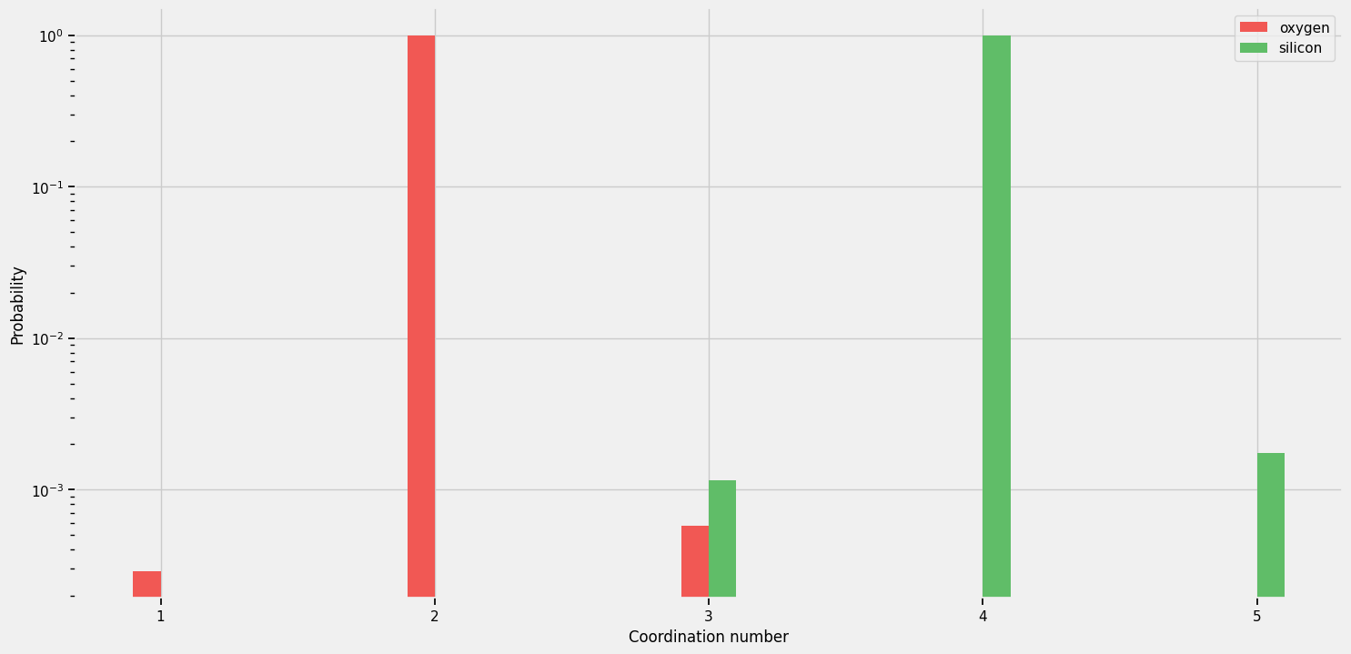
Interpretation:

• Almost all oxygen atoms have coordination number 2 (bridging oxygens connecting two SiO₄ tetrahedra). The rare CN = 1 and CN = 3 atoms are defects.

• Almost all silicon atoms have coordination number 4 (tetrahedral SiO₄ units). The rare CN = 3 and CN = 5 atoms are defects.

This silica glass has very little coordination-number disorder — nearly all atoms have the ideal coordination. This is typical of well-equilibrated silica glass.

However, BNE is not zero: the bond network is still disordered. The types of the ring environments vary from atom to atom. That real-space topological heterogeneity is what notebooks 3 and 4 measure.