Notebook 1 — Structure Preparation and Bonding

What is this tutorial about?

This notebook is the first in a series of six that walk you through computing Bond-Network Entropy (BNE) — a single number that measures how structurally disordered a material is at the level of its bond network.

We use silica glass (SiO₂) as our running example. Silica glass has very peaked (ordered) coordination number distribution (almost every Si is bonded to 4 oxygens; almost every O to 2 silicons), yet it is spatially disordered: the local environments have rings with irregular sizes and shapes. BNE is designed to capture exactly that kind of topological disorder.

---

The BNE pipeline — how the six notebooks fit together

Step	Notebook	What we compute
1	Notebook 1 (this one)	Interatomic distances; choice of bond cutoff
2	Notebook 2	Adjacency matrix; coordination numbers
3	Notebook 3	H₁ barcode for each atom’s local atomic environment (LAE)
4	Notebook 4	BNE = Shannon entropy of the barcode distribution across all atoms
5	5_BNE_workflow.py	Repeat for many LAE sizes 1–80 (run from the terminal), precomputed values available
6	Notebook 6	BNE growth rate and saturation as a function of LAE size

---

The structure file

We load a POSCAR file — the standard VASP format for atomic structures. It contains lattice vectors (the size and shape of the periodic simulation box) and atomic positions in fractional coordinates.

Our silica glass has 5184 atoms (3456 O + 1728 Si) in a cubic box of side ~42.8 Å. The structure is taken from the following reference (source: PNAS 2025).

Library + visualization setup

import os, sys

import numpy as np
import pandas as pd
import scipy
from scipy.constants import physical_constants

import ase
from ase.io import read, write

matplotlib_style = 'fivethirtyeight'
import matplotlib.pyplot as plt
plt.style.use(matplotlib_style)
import seaborn as sns
sns.set_context('notebook')


# see https://github.com/CamDavidsonPilon/Probabilistic-Programming-and-Bayesian-Methods-for-Hackers
# for inspiration and other tricks with visualization
class _Colors(object):
    """Helper class with different colors for plotting"""
    red = '#F15854'
    blue = '#5DA5DA'
    orange = '#FAA43A'
    green = '#60BD68'
    pink = '#F17CB0'
    brown = '#B2912F'
    purple = '#B276B2'
    yellow = '#DECF3F'
    gray = '#4D4D4D'
    cyan = '#00FFFF'
    rebecca_purple = '#663399'
    chartreuse = '#7FFF00'
    dark_red = '#8B0000'

    def __getitem__(self, i):
        color_list = [
            self.red,
            self.orange,
            self.green,
            self.blue,
            self.pink,
            self.brown,
            self.purple,
            self.yellow,
            self.gray,
            self.cyan,
            self.rebecca_purple,
            self.chartreuse,
            self.dark_red
        ]
        return color_list[i % len(color_list)]


Colors = _Colors()

from typing import Tuple, List
from tqdm import tqdm

Step 1 — Finding interatomic distances (Minimum Image Convention)

To decide which atoms are bonded we first need all pairwise distances.

Why is this tricky in a periodic structure? Atomistic simulations use periodic boundary conditions (PBC): the simulation box is tiled infinitely in all three directions. An atom near one face of the box can be bonded to an atom that appears on the opposite face — their true nearest-image distance is short even though their raw coordinate difference is large.

The Minimum Image Convention (MIC) gives the correct distance and is implemented in ASE: ASE’s atoms.get_distances(..., mic=True)

The function below computes, for every atom, the distances to its n_smallest nearest neighbours, sorted from closest to furthest. We store them as two arrays of shape (N_atoms, n_smallest):

• distances[i, k] — distance from atom \(i\) to its \(k\)-th nearest neighbour

• idx_distances[i, k] — global index of that neighbour

# read structure downloaded from https://www.pnas.org/doi/abs/10.1073/pnas.2422763122
filename = "./data/structural/silica_glass_5184_atoms/POSCAR"

atoms = read(filename)
atoms

Atoms(symbols='O3456Si1728', pbc=True, cell=[42.7702331357, 42.7702331357, 42.7702331357])

atomic_numbers = atoms.get_atomic_numbers()
atomic_numbers  # 8 is oxygen, 14 is silicon

array([ 8,  8,  8, ..., 14, 14, 14], shape=(5184,))

From atomic numbers, we can see that first 2/3 of indices are oxygen, last 1/3 is silicon, this will be used later

# handy function to obtain distances to nearest atoms (distances) and their indices (idx_distances)

def obtain_distances_ase(
    atoms: ase.atoms.Atoms,
    n_smallest: int,
) -> Tuple[np.ndarray, np.ndarray]:
    """
    Compute the n_smallest nearest-neighbour distances for every atom using
    the ASE Minimum Image Convention (preferred method).

    ASE's ``get_distances`` method handles the MIC correctly for all cell
    shapes (orthorhombic, monoclinic, triclinic), making it more accurate
    than the manual implementation for non-cubic cells.

    Parameters
    ----------
    atoms : ase.atoms.Atoms
        ASE Atoms object containing positions and cell (lattice vectors).
        Load from file with ``ase.io.read(filename)``.
    n_smallest : int
        Number of nearest neighbours (including central atom) to keep per atom.

    Returns
    -------
    distances : np.ndarray, shape (N, n_smallest)
        Sorted nearest-neighbour distances (in Ångström).
    idx_distances : np.ndarray, shape (N, n_smallest)
        Global atom indices corresponding to those distances.
    """

    distances = []
    idx_distances = []

    nat = len(atoms)
    atom_indices = np.arange(0, nat, 1)

    for k in tqdm(range(len(atoms)), desc="Distances"):

        # ASE computes MIC-corrected distances from atom k to all others
        distance = atoms.get_distances(k, atom_indices, mic=True)

        # keep only the n_smallest nearest neighbours using argpartition
        if n_smallest < nat:
            idx_distance = np.argpartition(distance, n_smallest)[:n_smallest]
        else:
            idx_distance = np.arange(0, nat, 1)

        # sort by distance within the selected neighbours
        idx_distance = idx_distance[np.argsort(distance[idx_distance])]

        idx_distances.append(idx_distance)
        distances.append(distance[idx_distance])

    distances = np.array(distances)
    idx_distances = np.array(idx_distances)
    return distances, idx_distances

Timing note: The cell below loops over all 5184 atoms and calls ASE’s MIC distance routine for each one. On a typical laptop this takes 15-30 seconds. The %%time magic will print the exact wall-clock time when it finishes. You only need to run this once per session — all later notebooks reuse the same computation.

%%time
distances, idx_distances = obtain_distances_ase(atoms, 300)

Distances: 100%|███████████████████████████████████████████████████████████████████████████████████████████████████████████████████████████████████████████████████████| 5184/5184 [00:13<00:00, 373.39it/s]

CPU times: user 11.6 s, sys: 4.52 s, total: 16.1 s
Wall time: 13.9 s

distances[0, :30]

array([0.        , 1.59823125, 1.59995058, 2.53651019, 2.55824096,
       2.57382612, 2.61360709, 2.64484089, 2.72432556, 3.12889256,
       3.33988123, 3.52683473, 3.66502544, 3.67642757, 3.7418959 ,
       3.81488167, 3.99920102, 4.03340691, 4.1437194 , 4.18815551,
       4.26071218, 4.35772077, 4.39811906, 4.4680171 , 4.53320779,
       4.60976551, 4.78718661, 4.83595509, 4.88701397, 4.98273803])

Step 2 — Reading the distance distribution

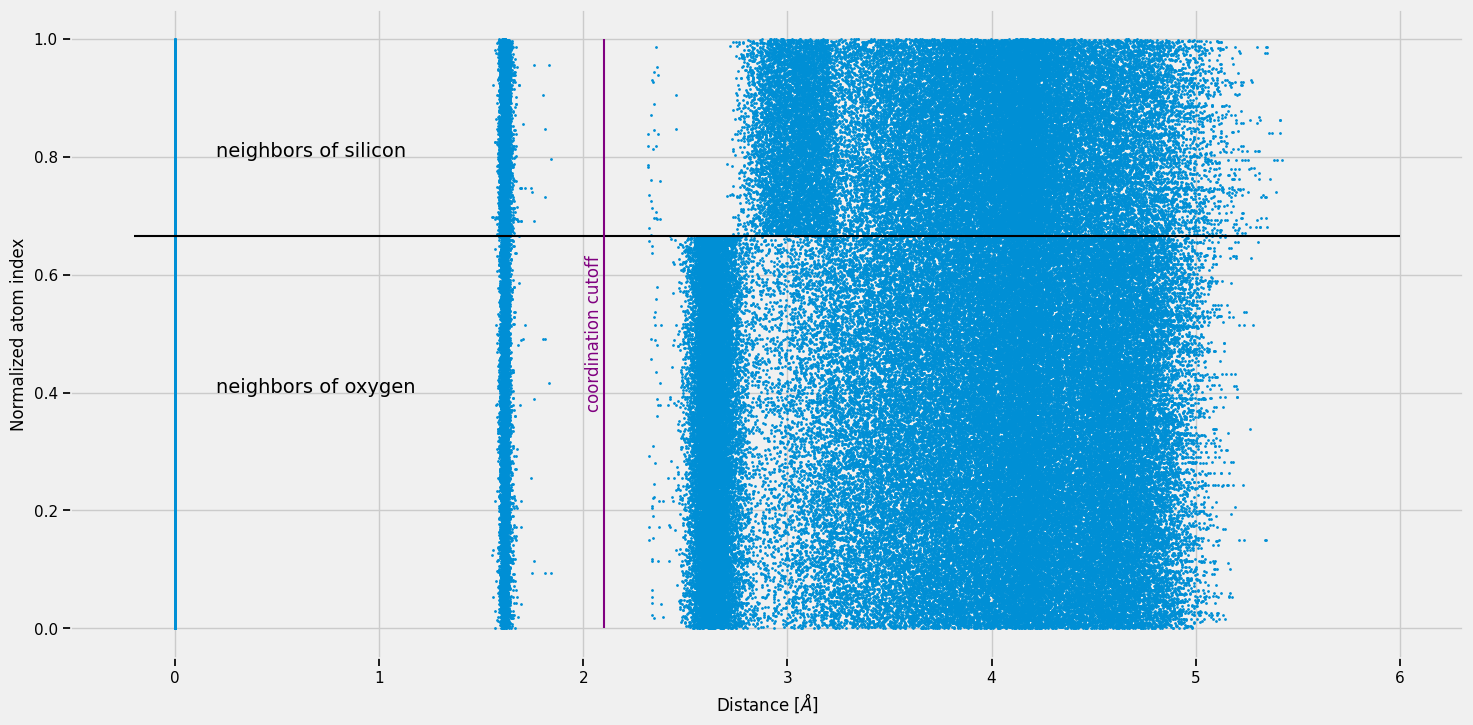
We plot the 30 nearest-neighbour distances for every atom as a scatter plot. Each point is one (atom, neighbour) pair. The y-axis is the normalised atom index (0 = first O, 1 = last Si), so the black horizontal line at 2/3 separates the oxygen atoms (below) from the silicon atoms (above).

We use a scatter plot rather than a histogram to show every data point without binning artefacts. Look for distinct vertical bands — these are coordination shells.

The purple vertical line marks our candidate bond cutoff at 2.1 Å.

plt.figure(figsize=(16, 8))

n_closest_neigh = 30

nat = len(atoms)
spectrum = np.linspace(0, 1, nat)
normalized_atomic_indices = np.repeat(spectrum, n_closest_neigh).reshape(nat, n_closest_neigh)

plt.scatter(distances[:, :n_closest_neigh], normalized_atomic_indices, s=1)



plt.hlines(2/3, -0.2, 6, color="black")

plt.text(0.2, 0.8, "neighbors of silicon", fontsize=14)
plt.text(0.2, 0.4, "neighbors of oxygen", fontsize=14)



plt.vlines(2.1, 0, 1, color='purple')

plt.text(2.05, 0.5, 'coordination cutoff',
        horizontalalignment='center',
        verticalalignment='center',
        rotation='vertical', color='purple')



plt.ylabel("Normalized atom index")
plt.xlabel(r"Distance [$\AA$]")

plt.show()

Let’s analyze the atom type of the neighbours

plt.figure(figsize=(16, 8))

n_closest_neigh = 30

nat = len(atoms)
spectrum = np.linspace(0, 1, nat)
normalized_atomic_indices = np.repeat(spectrum, n_closest_neigh).reshape(nat, n_closest_neigh)

vis_colors = {8:Colors[0], 14:Colors[2]} # oxygen is red, silicon is green

def apply_color(idx):
    return vis_colors[idx]

color_array = np.vectorize(apply_color)(atomic_numbers[idx_distances[:, :n_closest_neigh]])


plt.scatter(distances[:, :n_closest_neigh].flatten(), normalized_atomic_indices.flatten(), s=1, c=color_array.flatten())




plt.hlines(2/3, -0.2, 6, color="black")

plt.text(0.2, 0.9, "neighbors of silicon", fontsize=14)
plt.text(0.2, 0.4, "neighbors of oxygen", fontsize=14)

plt.text(0.3, 0.85, "Si-Si", fontsize=14, color=Colors[2])
plt.text(0.55, 0.85, "Si-O", fontsize=14, color=Colors[0])

plt.text(0.3, 0.35, "O-O", fontsize=14, color=Colors[0])
plt.text(0.55, 0.35, "O-Si", fontsize=14, color=Colors[2])




plt.vlines(2.1, 0, 1, color='purple')

plt.text(2.05, 0.5, 'coordination cutoff',
        horizontalalignment='center',
        verticalalignment='center',
        rotation='vertical', color='purple')


plt.ylabel("Normalized atom index")
plt.xlabel(r"Distance [$\AA$]")

plt.show()

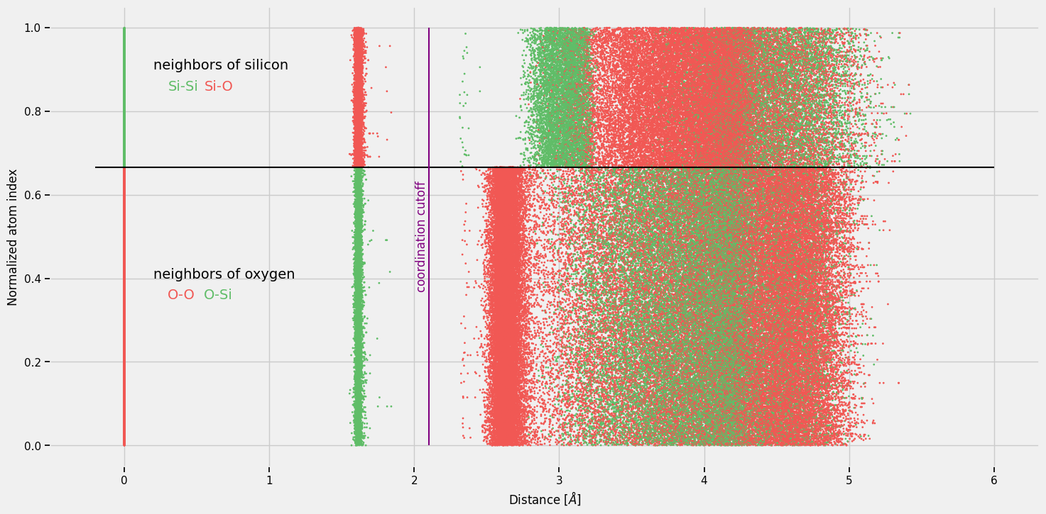
The cutoff of 2.1 Å (purple line) captures all Si–O nearest-neighbour bonds while excluding all Si–Si and O–O pairs — exactly what we want for the silica bond network. For adjacency matrix we will also remove self-distances (band at distance = 0.0 Å).

How to choose the cutoff for a different material

The cutoff r_c = 2.1 Å is specific to silica. For a new material, follow these steps:

1. Plot the distance distribution (as above). Look for a clear gap or valley between the first peak (nearest-neighbour bonds) and the second peak (next-nearest neighbours).

2. Place ``r_c`` inside that gap. For silica, Si–O bonds are ~1.6 Å and the first gap extends from ~1.9 Å to ~2.2 Å — any cutoff in that range works.

3. Some materials don’t have a single cutoff, and atom-dependent cutoffs might have to be used. The distance is also not always a good descriptor of whether atoms are bonded, electronic charge density might be a better descriptor in such cases, but this goes beyond the scope of this tutorial.

Considerations that change between materials:

• Bond lengths depend on the element pair. C–C bonds in amorphous carbon are ~1.3–1.6 Å; Si–O bonds in silica glass are ~1.6 Å

• Exclude second-shell atoms. Setting the cutoff too large inflates coordination numbers and distorts the ring topology that BNE measures.

• For multi-component systems, the distance plot coloured by atom type (above) is especially helpful for identifying which peaks correspond to which bond pairs.